Performance

The Backtracking algorithm's worst case runtime is bound by , the worst case only happens in an input instance when all the nodes in the tree are searched. comes from solving the recurrence relationship of the recursive algorithm as follows.

When we are at a leaf (a=n) worst case changelowest will need to be run every time, changelowest is in so the time is cn. Otherwise worst case we need to recurse 3 times adding one to a.

Change of variable to n.

multiplicity 2

This shows that the worst case running time is bound by , but that does not occur very often. Many things about the input instance can effect how fast the algorithm completes other than the number of tasks. One thing that I focused my research on was how the algorithm performed when I varied the cost between processors on one task. I created input instances randomly and varied the cost width by what range of random numbers could be picked. For instance if I let the task times be picked randomly between 1 and 10, the variance would be small while, if I let the task times be picked randomly between 1 and 1000, they tended to have a large variance.

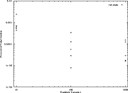
In the above logarithmic scale plot is data obtained from running the algorithm to schedule 21 tasks and varying the random variance it is plotted against the number of nodes in the tree that where examined as a percentage of all the nodes in the tree. You can see that there is a general decrease in the number of visited nodes when the tasks have larger variance as compared to small variance. Also over all the runs here only one even approaches visiting 0.5% of the total nodes in the tree.

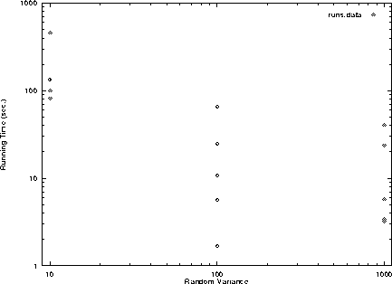
This logarithmic scale plot uses the same data as above, but shows the time taken to complete the scheduling against the variance size. Again you can see a general speedup when the variance increases in size.

From both of the last two plots I find that when the random variance is large, or that the input numbers are farther apart the algorithm performs better. This may happen because the partial schedules with larger variance can be ignored higher in the tree because sums can get larger than the best time so far earlier. When the tasks costs look a lot the same and cost about the same as their neighboring schedules the algorithm can not tell that one is certainly better than the next until very near the bottom of the tree. Conversely when there is larger difference between costs the better cost becomes more apparent higher in the tree making the search even smaller and thus comes the speedup. Although I don't think this speedup going to increase at the same rate as the the variance is increased, you can see from both plots that the speedup from 10 to 100 is generally greater than the speedup between 100 and 1000. So if the variance were 10000 next the speedup would not be very significant.

From smaller single run experiments I gained some more knowledge on how my algorithm performed. I created a input instance of 21 tasks where every task took a time 10 units on each processor, this instance took a significantly longer time to schedule than other 21 task instances. I believe this happened because at every leaf before it found what was to become the absolute best scheduling it found a new intermediate best. That run completed by looking at about 1% of all the nodes in the tree.

Another input instance I created of size 21 was designed so the only optimum scheduling was where all the tasks were run on the first processor. Once the first, and best, schedule was obtained by the algorithm, it eliminated all other schedules at every level of the recursion it left, effectively only looking at no other complete schedules. This run only looked at 64 nodes in a tree with about 15 billion nodes.

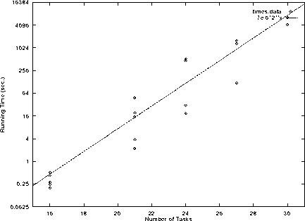
Above is a plot of the running time of the algorithm against the number of tasks to schedule. From playing around with some numbers I managed to fit a curve in to the data points. The is only from empirical data and has no meaning asymptotically, but it does show that the algorithm is still behaving in exponential time, and I imagine that there might be a large enough n that shows as the theoretical analysis suggests.