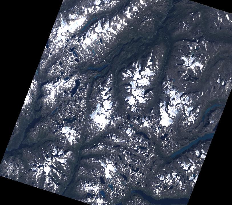
 This image show the "true colour" version, with the blue range
assigned to the blue colour, green range to green colour and red range
to red colour.
This image show the "true colour" version, with the blue range
assigned to the blue colour, green range to green colour and red range
to red colour.Assigment 8 in GEG2210 - Data Collection - Land Surveying, Remote Sensing and Digital Photogrammetry
By Petter Reinholdtsen and Shanette Dallyn, 2005-05-01.
This exercise was performed by logging into jern.uio.no using ssh and running ERDAS Imagine. Started by using 'imagine' on the command line. The images were loaded from /mn/geofag/gggruppe-data/geomatikk/
We tried to use svalbard/tm87.img, but it only have 5 bands. We decided to switch, and next tried jotunheimen/tm.img, which had 7 bands.
The pixel values in a given band is only a using a given range of values. This is because sensor data in a single image rarely extend over the entire range of possible values.
The peak values of the histograms represent the the spectral sensitivity values that occure the most often with in the image band being analysed.
This image show the "true colour" version, with the blue range
assigned to the blue colour, green range to green colour and red range
to red colour.
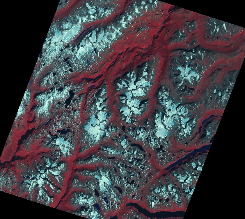
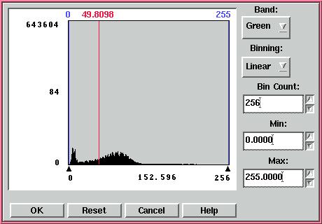 Water acts as an absorbing body so in the near infrared spectrum,
water features will appear dark or black meaning that all near
infrared bands are absorbed. On the other hand, land features
including ice, act as reflector bodies in this band. The histogram
show most values between 7 and 110. The mean is 40.1144. There are
two peaks at 7 and 40.
Water acts as an absorbing body so in the near infrared spectrum,
water features will appear dark or black meaning that all near
infrared bands are absorbed. On the other hand, land features
including ice, act as reflector bodies in this band. The histogram
show most values between 7 and 110. The mean is 40.1144. There are
two peaks at 7 and 40.
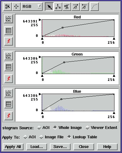
When we look at the linear contrast functions, we can move the slope and shift values increasing or decreasing the contrast of the image. For example, in the linear contrasting we moved the slope value from 1.00 to 3.00 to obtain a brighter appearing image, and then we moved the shift from 0 to 10 to recieve a sharper image.

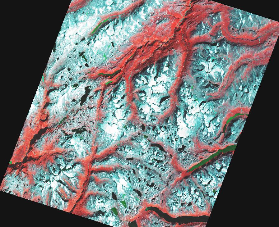
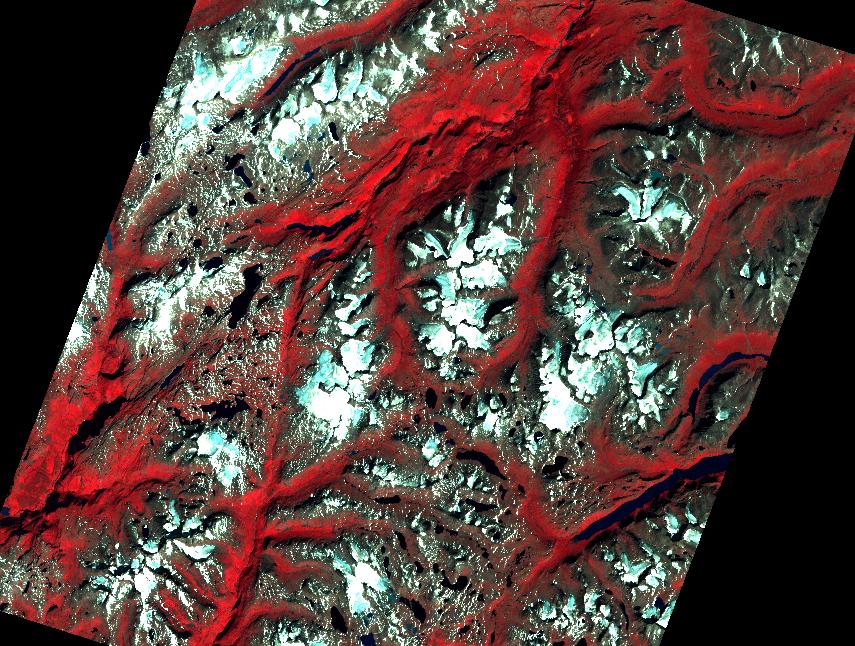
We also tried to do histogram equilization on the standard infrared composition. This changed the colours in the image, making the previously green areas red, and the brown areas more light blue. In this new image, we can clearly see the difference between two kind of water, one black and one green. We suspect the green water might be deeper, but do not know for sure.
We can get best contrast stretch by using the histogram
equalisation. This gave us the widest range of visible separation
between features.

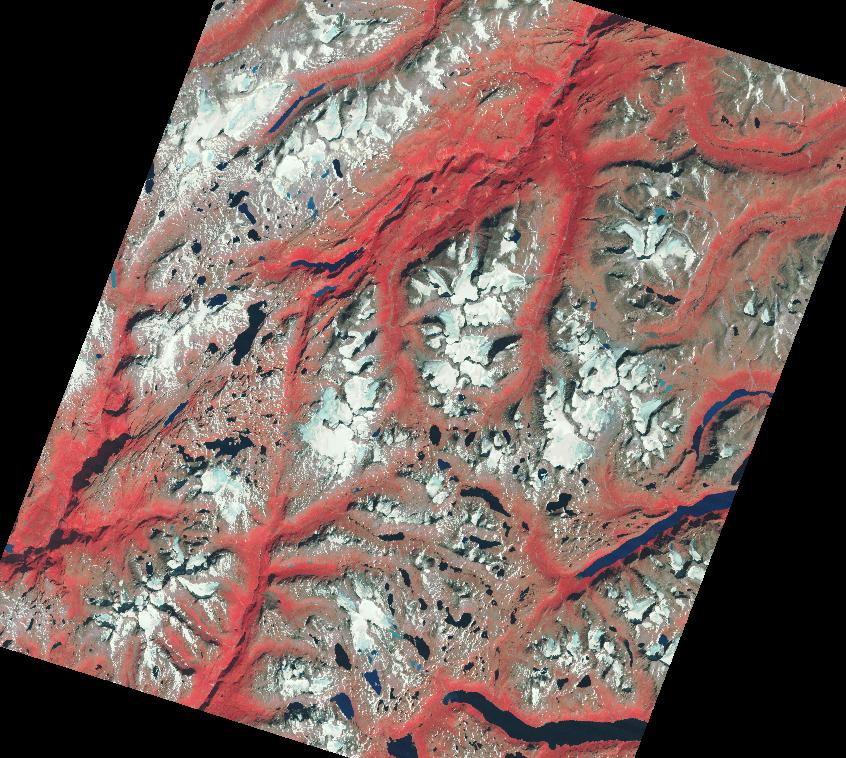
Comparing a map we found on the web, and the standard infrared image composition, we can identify some features from the colors used:
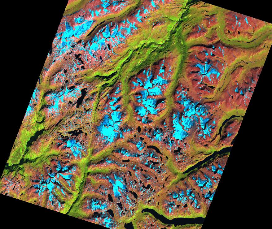
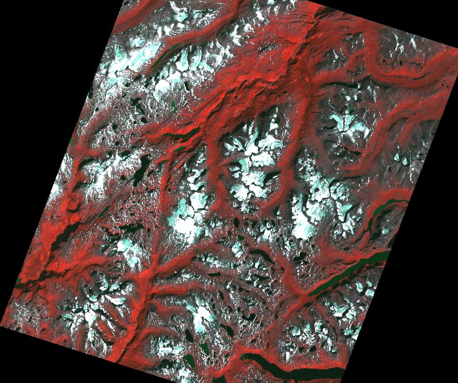
Next, we tried to shift the frequencies displayed to use blue for the red band, green for the near ir band and red for the mid ir (1.55-1.75 um). With this composition, we get some changes in the colours of different features:
 '
'
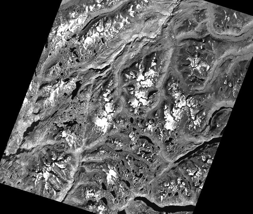
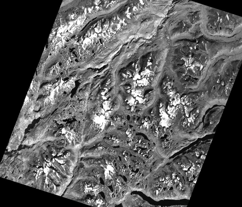
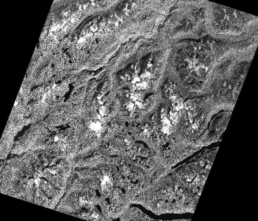
We decided to work on the grey scale version of the near infrared (band4). We changed the colour assignment to use this band for all three colours, giving us a gray scale image.
 '
'
We applied the 3x3 low pass filter on this image, and this gave us almost the same image as the original. If you look closely you can see that some white dots in the original disapper, and some of the water edges seem to blur very slightly.
 '
'
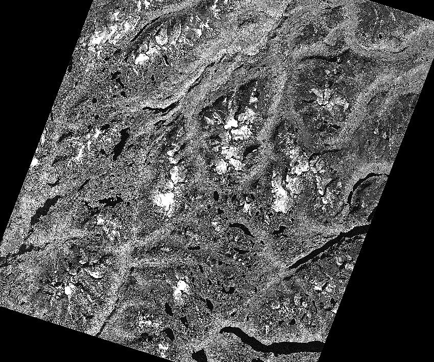
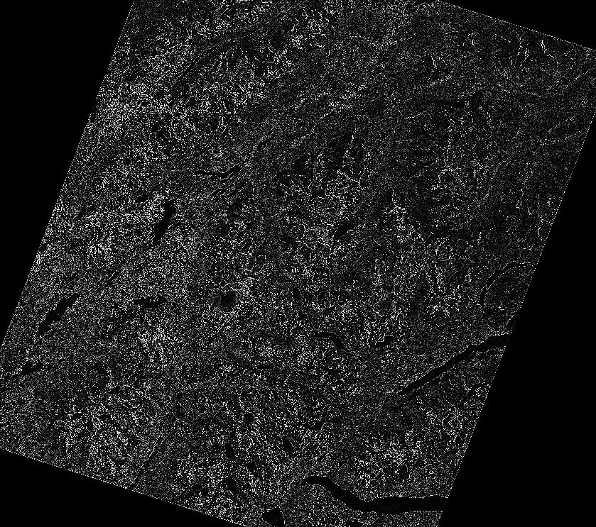
We also tried the 3x3 high pass filter on the band4 grey scale image. This gave a very noisy image. Edges of vallies and ice are not well defined. The black waters are still obvious.
 '
'
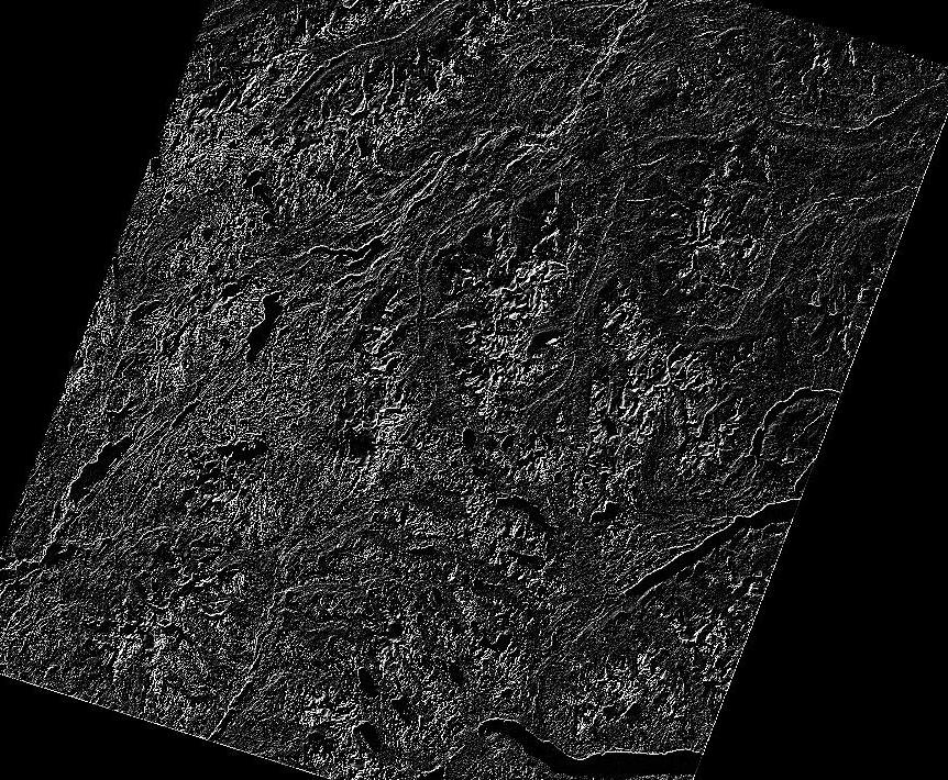
We also tried the 3x3 edge detection, and this gave us
an image that makes it difficult to distinguish elevation features
such as the valleys. Rather, edge detection allows us to study main
features in an area like the lakes. (insert band4 edge 3 image)
 '
'
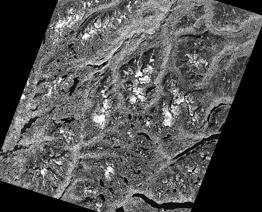
We tried a gradient filter using this 3x3 matrix. The matrix was chosen to make sure the sum of all the weights were zero, and to make sure the sum of horizontal, vertical and diagonal numbers were zero too.
| 1 | 2 | -1 |
| 2 | 0 | -2 |
| 1 | -2 | -1 |
The gradient filter used gave us enhancement on lines in the vertical, horizontal and diagonal directions. This is seen by the white lines that outline certain areas of main features like the rivers within the vallies and some of the lakes.
 '
'
When we rework the matrix to equal negative one, we end up with a lot of noise in the image that also seems to blurr the image. Using a negative one matrix is not optimal if you are trying to obtain sharpness.
| -1 | -1 | -1 |
| -1 | 7 | -1 |
| -1 | -1 | -1 |
 '
'
We then tried with a 3x3 matrix were the sum of all values equals 1, to enhance the high frequency parts of the image.
| -1 | -1 | -1 |
| -1 | 9 | -1 |
| -1 | -1 | -1 |
This gave us a sharper looking image compared to the result of the negative 1 filter. This is not really obvious unless one is comparing the two images carefully. In order to see more differences the matrix sums would have to be more then plus/minus one.